Week 10 Lab: Machine Learning Force Fields (ML-FF)
Contents
Week 10 Lab: Machine Learning Force Fields (ML-FF)
Student Name: YOUR NAME HERE
Preamble
Dataset needed
Before we begin, please start the download the dataset needed for training: QM dataset needed. This is a 4.48 GB
tarfile.Next, please decompress the
tarfile. This can be done on WinOS with 7zip, or Linux/Mac with the command$ tar -xf ANI1_release.tar.gz
Packages needed
# This cell will install any of the missing packages we'll use in the notebook
import sys
!{sys.executable} -m pip install torch
!{sys.executable} -m pip install torchani
!{sys.executable} -m pip install tqdm
!{sys.executable} -m pip install tensorboard
!{sys.executable} -m pip install h5py
ML-FF: ANI-1 exercise
%matplotlib inline
Train Your Own Neural Network Potential
This example shows how to use TorchANI to train a neural network potential
with the setup identical to NeuroChem. We will use the same configuration as
specified in inputtrain.ipt.
Note
TorchANI provide tools to run NeuroChem training config file `inputtrain.ipt`. See: `neurochem-training`.
Warning
The training setup used in this file is configured to reproduce the original research at "Less is more: Sampling chemical space with active learning" (https://aip.scitation.org/doi/10.1063/1.5023802) as much as possible. That research was done on a different platform called NeuroChem which has many default options and technical details different from PyTorch. Some decisions made here (such as, using NeuroChem's initialization instead of PyTorch's default initialization) is not because it gives better result, but solely based on reproducing the original research. This file should not be interpreted as a suggestions to the readers on how they should setup their models.
To begin with, let’s first import the modules and setup devices we will use:
import torch
import torchani
import os
import math
import torch.utils.tensorboard
import tqdm

# helper function to convert energy unit from Hartree to kcal/mol
from torchani.units import hartree2kcalmol

# device to run the training
device = torch.device('cuda' if torch.cuda.is_available() else 'cpu')
Now let’s setup constants and construct an Atomic Environment Vector (AEV) computer.
These numbers can be found in
rHCNO-5.2R_16-3.5A_a4-8.params.The atomic self energies given in
sae_linfit.datare computed from ANI-1x dataset. These constants can be calculated for any given dataset ifNoneis provided as an argument to the object of :class:EnergyShifterclass.
Note
Besides defining these hyperparameters programmatically, :mod:`torchani.neurochem` provide tools to read them from file.
These parameters have suffix
rfor the radial andafor angular functions (See equations 3 and 4 ofsmith2017-1).
Rcr = 5.2000e+00
Rca = 3.5000e+00
EtaR = torch.tensor([1.6000000e+01], device=device)
ShfR = torch.tensor([9.0000000e-01, 1.1687500e+00, 1.4375000e+00, 1.7062500e+00, 1.9750000e+00, 2.2437500e+00, 2.5125000e+00, 2.7812500e+00, 3.0500000e+00, 3.3187500e+00, 3.5875000e+00, 3.8562500e+00, 4.1250000e+00, 4.3937500e+00, 4.6625000e+00, 4.9312500e+00], device=device)
Zeta = torch.tensor([3.2000000e+01], device=device)
ShfZ = torch.tensor([1.9634954e-01, 5.8904862e-01, 9.8174770e-01, 1.3744468e+00, 1.7671459e+00, 2.1598449e+00, 2.5525440e+00, 2.9452431e+00], device=device)
EtaA = torch.tensor([8.0000000e+00], device=device)
ShfA = torch.tensor([9.0000000e-01, 1.5500000e+00, 2.2000000e+00, 2.8500000e+00], device=device)
species_order = ['H', 'C', 'N', 'O']
num_species = len(species_order)
aev_computer = torchani.AEVComputer(Rcr, Rca, EtaR, ShfR, EtaA, Zeta, ShfA, ShfZ, num_species)
energy_shifter = torchani.utils.EnergyShifter(None)
Remember the modified Behler-Parrinello functions from last lecture:
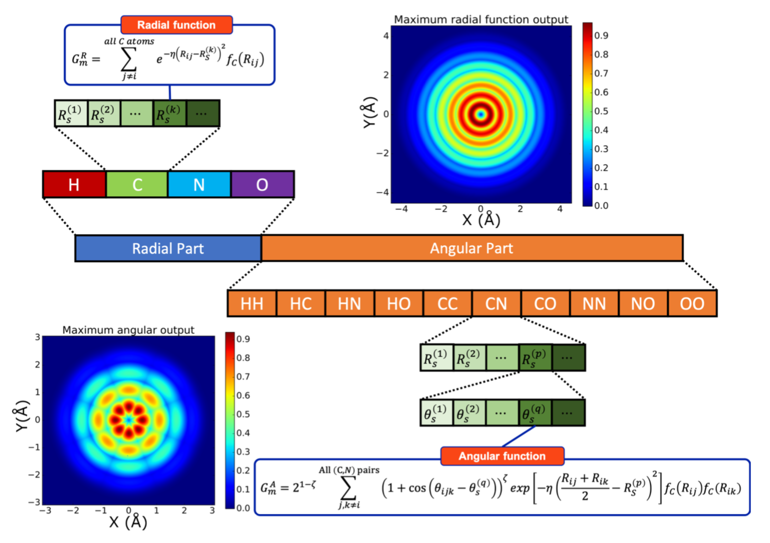
where
The correspondence is as follows:
Rcr: The \(R_C\) value in the \(f_C\) term for the radial functions (Å)Rca: The \(R_C\) value in the \(f_C\) term for the angular functions (Å)EtaR: A set of \(\eta\) values to use for the radial functions (Å\(^{-2}\))ShfR: A set of \(R_s^{(k)}\) values (“shifts”) to use for the radial functions (Å)Zeta: A set of \(\zeta\) values to use in the angular functionsShfZ: A set of \(\theta_s^{(q)}\) values to use in the angular functions (radians)EtaA: A set of \(\eta\) values to use for the angular functions (Å\(^{-2}\))ShfA: A set of \(R_s^{(p)}\) values (“shifts”) to use for the angular functions (Å)
Setting up your datasets
Now let’s setup datasets. These paths assumes the user run this script under the
examplesdirectory of TorchANI’s repository. If you download this script, you should manually set the path of these files in your system before this script can run successfully.Also note that we need to subtracting energies by the self energies of all atoms for each molecule. This makes the range of energies in a reasonable range. The second argument defines how to convert species as a list of string to tensor, that is, for all supported chemical symbols, which is correspond to
0, which correspond to1, etc.See this Dataset description for a explanation and details of this dataset.
WARNING
Please fix the variable
pathprefixfor your system. It must be the path to the folder containing the ANIh5files (the ones from the 4.48 GBtarfile linked at the beginning).
#Additional#
pathprefix = "./ANI-1_release/"
#Additional#
# Check if the files are in the folder (only check for the first one)
import os.path
if not os.path.isfile(os.path.join(pathprefix,"ani_gdb_s01.h5")):
    print("Can't find the ANI h5 files in folder "+pathprefix)
    for i in range(5):
        print("^")
else:
    print("ANI h5 files located!")
try:
    path = os.path.dirname(os.path.realpath(__file__))
except NameError:
    path = os.getcwd()
#dspath = os.path.join(path, '../dataset/ani1-up_to_gdb4/ani_gdb_s01.h5') # <- Original line:
dspath = os.path.join(path, pathprefix+'/ani_gdb_s01.h5')
batch_size = 2560

# Additional#: Here the dataset is split into training and validation set
training, validation = torchani.data.load(dspath).subtract_self_energies(energy_shifter, species_order).species_to_indices(species_order).shuffle().split(0.8, None)
training = training.collate(batch_size).cache()
validation = validation.collate(batch_size).cache()
print('Self atomic energies: ', energy_shifter.self_energies)
When iterating the dataset, we will get a dict of name->property mapping
Now let’s define atomic neural networks.
Setting up your Architecture
Additional# Here the different neural networks (one for each atom) are initialized.
The even-index elements of the NNs are the hidden layers. For example,
torch.nn.Linear(160, 128)means that the previous layer has 160 neurons and the current layer has 128 neurons.The odd-index elements are the activation functions. The function used is the ‘Continuously differentiable Exponential Linear Units’ (CELU), see https://pytorch.org/docs/stable/generated/torch.nn.CELU.html#torch.nn.CELU
Its argument is the alpha value of the CELU formulation (not related to the learning rate)
aev_dim stores the length (384) of the atomic environment vectors (AEV). See section 2.2 of smith2017-1. (Note: Said paper, in page 9, says that the AEVs have length 768. The AEVs were later shortened to 368 without loss of accuracy)
All 4 neural networks are loaded on nn for optimization.
aev_dim = aev_computer.aev_length

H_network = torch.nn.Sequential(
    torch.nn.Linear(aev_dim, 160),
    torch.nn.CELU(0.1),
    torch.nn.Linear(160, 128),
    torch.nn.CELU(0.1),
    torch.nn.Linear(128, 96),
    torch.nn.CELU(0.1),
    torch.nn.Linear(96, 1)
)

C_network = torch.nn.Sequential(
    torch.nn.Linear(aev_dim, 144),
    torch.nn.CELU(0.1),
    torch.nn.Linear(144, 112),
    torch.nn.CELU(0.1),
    torch.nn.Linear(112, 96),
    torch.nn.CELU(0.1),
    torch.nn.Linear(96, 1)
)

N_network = torch.nn.Sequential(
    torch.nn.Linear(aev_dim, 128),
    torch.nn.CELU(0.1),
    torch.nn.Linear(128, 112),
    torch.nn.CELU(0.1),
    torch.nn.Linear(112, 96),
    torch.nn.CELU(0.1),
    torch.nn.Linear(96, 1)
)

O_network = torch.nn.Sequential(
    torch.nn.Linear(aev_dim, 128),
    torch.nn.CELU(0.1),
    torch.nn.Linear(128, 112),
    torch.nn.CELU(0.1),
    torch.nn.Linear(112, 96),
    torch.nn.CELU(0.1),
    torch.nn.Linear(96, 1)
)

nn = torchani.ANIModel([H_network, C_network, N_network, O_network])
print(nn)
Initialize the weights and biases.
Note
Pytorch default initialization for the weights and biases in linear layers is Kaiming uniform. See: `TORCH.NN.MODULES.LINEAR`_ We initialize the weights similarly but from the normal distribution. The biases were initialized to zero.
https://pytorch.org/docs/stable/_modules/torch/nn/modules/linear.html#Linear
Additional# The Kaiming distribution improves the training of a DNN that uses a ReLU-type (unbounded) activation function rather than sigmoid-type (within the interval (-1,1) or (0,1) ). For a complete account on the topic, see https://towardsdatascience.com/weight-initialization-in-neural-networks-a-journey-from-the-basics-to-kaiming-954fb9b47c79 .
This other read is not as didactic but derives the Kaiming initialization https://medium.com/@shoray.goel/kaiming-he-initialization-a8d9ed0b5899
def init_params(m):
    if isinstance(m, torch.nn.Linear):
        torch.nn.init.kaiming_normal_(m.weight, a=1.0)
        torch.nn.init.zeros_(m.bias)


nn.apply(init_params)
Let’s now create a pipeline of AEV Computer –> Neural Networks.
model = torchani.nn.Sequential(aev_computer, nn).to(device)
Now let’s setup the optimizers. NeuroChem uses Adam with decoupled weight decay to updates the weights and Stochastic Gradient Descent (SGD) to update the biases. Moreover, we need to specify different weight decay rate for different layers.
Note
The weight decay in `inputtrain.ipt`_ is named "l2", but it is actually not L2 regularization. The confusion between L2 and weight decay is a common mistake in deep learning. See: `Decoupled Weight Decay Regularization`_ Also note that the weight decay only applies to weight in the training of ANI models, not bias.
Setting up the Optimization Functions
Here the optimization is set up.
Only the even-index elements are selected since the odd elements are the activation functions.
The Adam(s) algorithm.
The weights are optimized by AdamW, a variant of the Adam optimization method.
A good introduction to the Adam Optimizer
The original paper Adam paper
A more general overview of gradient descent methods, which includes SGD and the Adam variants.
A few points about Adam:
it can be seen as an extension of SGD.
the method is called Adam (not A.D.A.M. or such). The name is derived from ADAptive Moment estimation.
easy to implement and understand.
appropriate for problems with large amounts of data, parameters, and noisy/sparse gradients.
SGD uses one learning rate for all parameters; Adam uses one for each parameter.
It’s a refinement of the momentum optimization method.
The momentum method emulates a ball moving in a ravine: the ball’s future position depends on the ravine’s gradient AND on the ball’s momentum.
The momentum method updates its parameters by \begin{equation} \Delta \theta_i(t) = \alpha \cdot \Delta \theta_i(t-1) - \epsilon \frac{\partial J}{\partial \theta_i}(t) \end{equation}
\(\Delta \theta_i\) is the change in the parameter \(\theta_i\) for the epoch \(t\).
\(\alpha\) is the momentum hyperparameter, usually \(\in [0.5,0.9]\).
\(\Delta \theta_i(t-1)\) is the previous change on \(\theta_i\).
\(\epsilon\) is the learning rate.
\(\partial J/\partial \theta_i\) is the derivative of the cost function wrt \(\theta_i\) for the current epoch.
It can be seen in the equation above that the Momentum method updates the model’s parameters using the rolling average of the gradient across the previous iterations, instead of relying solely in the current gradient.
The Adam method takes these refinements one step further, as it not only stores the rolling average of the gradient, denoted above as \(\alpha \cdot \Delta \theta_i(t-1)\), but also the rolling average of the squared gradient. It uses both to tweak each parameter’s learning rate separately. For a deeper explanation of the method, see section 4.6 of the gradient descent review or alternatively the original Adam paper.
Finally, the AdamW method is a variant of Adam that includes a decoupled weight decay. According to the authors,
we propose a simple modification to recover the original formulation of weight decay regularization by decoupling the weight decay from the optimization steps taken w.r.t. the loss function.
We provide empirical evidence that our proposed modification…(ii) substantially improves Adam’s generalization performance, allowing it to compete with SGD with momentum on image classification datasets (on which it was previously typically outperformed by the latter).
For a deeper explanation, see the authors’ paper.
Note that the biases below are optimized by SGD.
AdamW = torch.optim.AdamW([
    # H networks
    {'params': [H_network[0].weight]},
    {'params': [H_network[2].weight], 'weight_decay': 0.00001},
    {'params': [H_network[4].weight], 'weight_decay': 0.000001},
    {'params': [H_network[6].weight]},
    # C networks
    {'params': [C_network[0].weight]},
    {'params': [C_network[2].weight], 'weight_decay': 0.00001},
    {'params': [C_network[4].weight], 'weight_decay': 0.000001},
    {'params': [C_network[6].weight]},
    # N networks
    {'params': [N_network[0].weight]},
    {'params': [N_network[2].weight], 'weight_decay': 0.00001},
    {'params': [N_network[4].weight], 'weight_decay': 0.000001},
    {'params': [N_network[6].weight]},
    # O networks
    {'params': [O_network[0].weight]},
    {'params': [O_network[2].weight], 'weight_decay': 0.00001},
    {'params': [O_network[4].weight], 'weight_decay': 0.000001},
    {'params': [O_network[6].weight]},
])

SGD = torch.optim.SGD([
    # H networks
    {'params': [H_network[0].bias]},
    {'params': [H_network[2].bias]},
    {'params': [H_network[4].bias]},
    {'params': [H_network[6].bias]},
    # C networks
    {'params': [C_network[0].bias]},
    {'params': [C_network[2].bias]},
    {'params': [C_network[4].bias]},
    {'params': [C_network[6].bias]},
    # N networks
    {'params': [N_network[0].bias]},
    {'params': [N_network[2].bias]},
    {'params': [N_network[4].bias]},
    {'params': [N_network[6].bias]},
    # O networks
    {'params': [O_network[0].bias]},
    {'params': [O_network[2].bias]},
    {'params': [O_network[4].bias]},
    {'params': [O_network[6].bias]},
], lr=1e-3)
Setting up a learning rate scheduler to do learning rate decay
AdamW_scheduler = torch.optim.lr_scheduler.ReduceLROnPlateau(AdamW, factor=0.5, patience=100, threshold=0)
SGD_scheduler = torch.optim.lr_scheduler.ReduceLROnPlateau(SGD, factor=0.5, patience=100, threshold=0)
Train the model by minimizing the MSE loss, until validation RMSE no longer improves during a certain number of steps, decay the learning rate and repeat the same process, stop until the learning rate is smaller than a threshold.
We first read the checkpoint files to restart training. We use latest.pt
to store current training state.
latest_checkpoint = 'latest.pt'
Resume training from previously saved checkpoints:
if os.path.isfile(latest_checkpoint):
    checkpoint = torch.load(latest_checkpoint)
    nn.load_state_dict(checkpoint['nn'])
    AdamW.load_state_dict(checkpoint['AdamW'])
    SGD.load_state_dict(checkpoint['SGD'])
    AdamW_scheduler.load_state_dict(checkpoint['AdamW_scheduler'])
    SGD_scheduler.load_state_dict(checkpoint['SGD_scheduler'])
During training, we need to validate on validation set and if validation error is better than the best, then save the new best model to a checkpoint
def validate():
    # run validation
    mse_sum = torch.nn.MSELoss(reduction='sum')
    total_mse = 0.0
    count = 0
    for properties in validation:
        species = properties['species'].to(device)
        coordinates = properties['coordinates'].to(device).float()
        true_energies = properties['energies'].to(device).float()
        _, predicted_energies = model((species, coordinates))
        total_mse += mse_sum(predicted_energies, true_energies).item()
        count += predicted_energies.shape[0]
    return hartree2kcalmol(math.sqrt(total_mse / count))
We will also use TensorBoard to visualize our training process
tensorboard = torch.utils.tensorboard.SummaryWriter()
Training
Finally, we come to the training loop.
In this tutorial, we are setting the maximum epoch to a very small number, only to make this demo terminate fast. For serious training, this should be set to a much larger value
#Additional# Run the code in this cell if you want to restart the training from zero
import os
try:
    os.remove("best.pt")
    os.remove("latest.pt")
except:
    pass
mse = torch.nn.MSELoss(reduction='none')

print("training starting from epoch", AdamW_scheduler.last_epoch + 1)
max_epochs = 10
early_stopping_learning_rate = 1.0E-5
best_model_checkpoint = 'best.pt'

# Additional# This is the big loop for optimization
for _ in range(AdamW_scheduler.last_epoch + 1, max_epochs):
    rmse = validate()
    print('RMSE:', rmse, 'at epoch', AdamW_scheduler.last_epoch + 1)

    learning_rate = AdamW.param_groups[0]['lr']

    if learning_rate < early_stopping_learning_rate:
        break

    # checkpoint
    if AdamW_scheduler.is_better(rmse, AdamW_scheduler.best):
        torch.save(nn.state_dict(), best_model_checkpoint)

    # Additional# OPTIMIZATION HAPPENS HERE v
    AdamW_scheduler.step(rmse)
    SGD_scheduler.step(rmse)

    tensorboard.add_scalar('validation_rmse', rmse, AdamW_scheduler.last_epoch)
    tensorboard.add_scalar('best_validation_rmse', AdamW_scheduler.best, AdamW_scheduler.last_epoch)
    tensorboard.add_scalar('learning_rate', learning_rate, AdamW_scheduler.last_epoch)

    for i, properties in tqdm.tqdm(
        enumerate(training),
        total=len(training),
        desc="epoch {}".format(AdamW_scheduler.last_epoch)
    ):
        species = properties['species'].to(device)
        coordinates = properties['coordinates'].to(device).float()
        true_energies = properties['energies'].to(device).float()
        num_atoms = (species >= 0).sum(dim=1, dtype=true_energies.dtype)
        _, predicted_energies = model((species, coordinates))

        # Additional# Compute the loss function
        loss = (mse(predicted_energies, true_energies) / num_atoms.sqrt()).mean()

        AdamW.zero_grad()
        SGD.zero_grad()
        loss.backward()
        AdamW.step()
        SGD.step()

        #print("nn", nn.state_dict())
        #print("AdamW", AdamW.state_dict())

        # write current batch loss to TensorBoard
        tensorboard.add_scalar('batch_loss', loss, AdamW_scheduler.last_epoch * len(training) + i)
        #print("loss",loss) # custom

    torch.save({
        'nn': nn.state_dict(),
        'AdamW': AdamW.state_dict(),
        'SGD': SGD.state_dict(),
        'AdamW_scheduler': AdamW_scheduler.state_dict(),
        'SGD_scheduler': SGD_scheduler.state_dict(),
    }, latest_checkpoint)
Lab Question 1
As reported in the
smith2017-1paper (page 9, just above section 4), the RMSE for the training set is of just 1.2 kcal/mol. How close can you get using this notebook?
Lab Question 2 (bonus)
The method state_dict() can be used to display all the data contained in nn, AdamW, AdamW_scheduler, SGD, and SGD_scheduler.
In order to display a particular set of data, see below
nn.state_dict()
AdamW.state_dict()
AdamW_scheduler.state_dict()
SGD_scheduler.state_dict()
A key can be added to state_dict(), thus extracting a particular piece of information of the objects. For example,
SGD_scheduler.state_dict()['best']
SGD_scheduler.state_dict()['eps']
In particular, the weights of any layer of any element can be obtained by this method.
These keys have the format atNumber.layNumber.weight
atNumberrefers to the atom:0is H,1C,2N,3OlayNumberrefers to the layer:0means the first hidden layer,2the second,4the third,6the fourth (since the odd numbers store the activation functions)
The weights can be exported to a file using numpy. Its size can be known by the shape method.
nn.state_dict()['0.0.weight'] # First hidden layer of H (connects input layer and first hidden layer)
nn.state_dict()['0.2.weight'] # Second hidden layer of H (connects first hidden layer and second)
nn.state_dict()['0.0.weight'].shape
The cells below export all weights and biases to text files
if not os.path.exists("Weights-ANI"):
    os.mkdir("Weights-ANI")
import numpy as np
nElements = 4
listSymbols = [ 'H', 'C', 'N', 'O']
listIndicesLayers = [ 0, 2, 4, 6]
for i in range(nElements):
    for j in range(nElements):
        weightsSave = nn.state_dict()[str(i)+'.'+str(listIndicesLayers[j])+'.weight']
        np.savetxt('Weights-ANI/weight-'+listSymbols[i]+'-layer'+str(j+1)+'.dat',weightsSave)
        biasSave = nn.state_dict()[str(i)+'.'+str(listIndicesLayers[j])+'.bias']
        np.savetxt('Weights-ANI/bias-'+listSymbols[i]+'-layer'+str(j+1)+'.dat',biasSave)
Lab Question 3 (bonus)
Make a plot of predicted vs. calculated energies for one of the training sets.
Hint: look at the code in the training loop, and use training[i] instead of properties.
# your code here
Bibliography:
This document is based on the notebook found in https://aiqm.github.io/torchani-test-docs/examples/nnp_training.html. However, in this exercise, we add some additional explanations and exercises about ANI that will help the student understand the topic better and can be linked to the lecture better.
smith2017-1refers to the ANI-1 paper, available at https://doi.org/10.1039/C6SC05720A.Other references are included throughout the notebook as direct links