Week 01 Lab: Python Refresher Course
Contents
Week 01 Lab: Python Refresher Course
Student Name: YOUR NAME HERE

Before we start our 4-week machine learning content, we thought we should take some time to make sure everyone has the necessary tools and background knowledge. While a lot of the upcoming content will be heavily scaffolded with pre-written code, ideally by the end of this course you will not only be able to fully understand what this code is doing and how it works, but also be able to adapt these tools to your own purposes and even create and share your own tools with the scientific community.
Today we will learn (or practice) the following:
Shortcuts for working with jupyter notebooks
Installing and importing packages
Creating, manipulating, reading and writing Numpy arrays
Object oriented programming: Defining classes
For this class we will be working in pairs. Each pair will be working in their own Zoom breakout room. Remember to work together as you go through the notebook! If you have questions or difficulties either come back to the main session or use the “ask for help” Zoom function.
Part 1: Shortcuts for working with Jupyter notebooks
As you’ve already seen, Jupyter notebooks are great ways to combine code, formatted text, images, and even YouTube videos together into a single interactive document.
There are some keyboard shortcuts that make working in Jupyter much easier and learning them now will save you a lot of time in the long run!
Running cells
Click on the cell below and press Shift+Enter
# some python code
x = 2
y = x*10
print('y equals',y)
This is the most common way to traverse through notebooks: holding down the Shift key and executing the cells one at a time.
Execute the cells below and notice the asterisks on the left hand side
# more python code
from time import sleep
sleep(10)
print("Finally...")
# this cell won't run until the one above finishes
print("That took a while..")
Cells are run one at a time. An asterisk denotes either that a cell is currently being executed, or it is waiting for another cell to finish. Cells can be executed in any order and the number that appears on the left indicates the order in which it was executed.
Double click on the Markdown cell below to see its “code” and then “run” it with Shift+Enter
Check out this picture of a penguin!

Markdown cells can be edited and run just like code cells.
Manipulating cells
When working on a notebook often you want to create a new cell, change its type (e.g. “Code” to “Markdown”), move it, or delete it entirely. While there are tools to do these things in the menu above, there are also useful keyboard shortcuts that you should learn.
Use the Esc key on the cell below to change into “Command Mode”. The box surrounding the cell should turn blue.
Then go back to “Edit Mode” by pressing Enter. The box should turn green.
# some python code
a,b = 2,3
When you are in Edit Mode you can (obviously) edit the cells, add and remove text, etc. In Command Mode you can do things like the following:
Add a cell above this one (a)
Add a cell below this one (b)
Remove this cell (x)
Copy this cell (c)
Paste this cell (v)
Open up a help screen that tells you all of this and more! (h)
Make three empty cells below, write some code in each, copy the middle one and paste it, then delete them all
Part 2: Installing and importing packages, finding documentation and source code
A great thing about the Python language is that we can make use of a whole world of packages for numerical analysis, data visualization, statistics and machine learning. There are also a number of great packages for analysing biomolecular data, performing and analyzing molecular dynamics simulations, and even (as we saw on Tuesday) visualize biomolecular structures directly in Jupyter notebooks! This truly lets us stand on the shoulders of giants.

Importing packages
Say we want to solve the linear equation:
\begin{equation} {\bf A}{\bf x} = {\bf B} \end{equation}
where \({\bf A}\) and \({\bf B}\) are known matrices and \(x\) is unknown. We can do this by importing a particular package from scipy:
from scipy.linalg import solve
Note that if you see a message like: ModuleNotFoundError: No module named 'scipy' then this indicates scipy has not been installed or is not accessible to this Python kernel.
Installing packages
To install a new package you should use a package manager such as pip or conda using the command line. To make these new packages accessible you should shutdown and restart the server running the Jupyter notebook.
However, there is a shortcut: in Jupyter notebooks (and on Google Colab) you can run command line commands without leaving the notebook:
# no need to run this if you already have scipy
!pip install scipy
Any command that starts with “!” is run in the command line. Try out some other bash commands below such as pwd, ls -ltr and top.
# try out some bash commands
Finding documentation
Back to our linear equation example. Now that we imported the solve function, what if we forget how to format the inputs? Or we want to know which options are available when we call it? This information is in the documentation for this function, also known as the “doc string”. Documentation is of course available on the scipy webpage (found here), but again there is a shortcut:
solve?
Adding a question mark to any function or object will bring up the doc string for that object. It also works with user-defined functions:
def my_function(a):
    """This function returns the square of a number."""
    return a**2
my_function?
Examining source code
What if we want to see the source code? Well you could look at the bottom of the docstring to find the location of the file on your computer, open the file in a text editor, and search for the corresponding function name. But as you probably guessed, there is an easier way! Just add another question mark:
solve??
Scrolling down past the call signature and the docstring shows the source code of this function.
Part 3: Working with Numpy arrays
One library that is going to be indispensible in this course (and in most of scientific computing) is called numpy. This provides a convenient structure for organizing large sets of data of the same datatype (e.g. integers or floats) into single objects called “arrays”.
These arrays can be one-dimensional (like vectors), two-dimensional (like matrices) or have three or more dimensions. Each dimension of the array is also referred to as an “axis”.
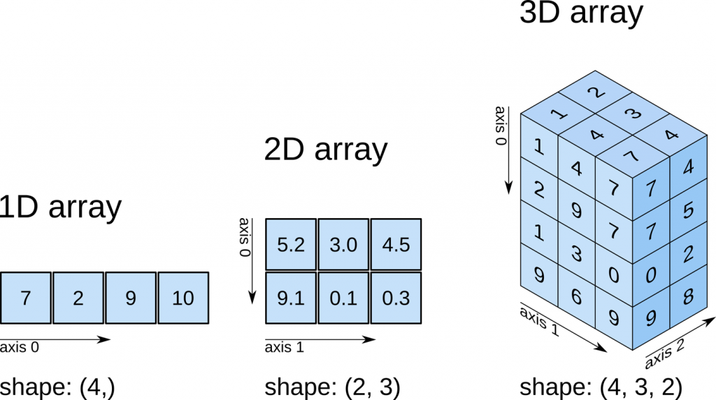
The size of an array along each axis is revealed by its “shape”, which is a list of integers, the first integer giving the shape along axis 0, the second integer giving the shape along axis 1, and so on.
The length of the shape list reveals the “dimensionality” of the array.
Numpy basics
Here are some YouTube videos made by the CMSE 201 team at MSU that give some background on Numpy arrays and multi-dimensional Numpy arrays:
# Numpy basics

from IPython.display import YouTubeVideo
YouTubeVideo("g7epZeDA_lQ",width=640,height=360)
# Mathematical operations with Numpy

from IPython.display import YouTubeVideo
YouTubeVideo("V2C9expTF1o",width=640,height=360)
Turn the following list into a numpy array, square all of the elements and print out the sum of the squares.
Hint: summing an array can be done easily with the .sum() function
import numpy as np

some_list = [1.6,8,3,1,22,64.7]
Check: the sum should be 4746.65
Manipulating multidimensional arrays
Here’s another CMSE 201 video describing two-dimensional arrays:
from IPython.display import YouTubeVideo
YouTubeVideo("KXPtg7iHbfw",width=640,height=360)
Much of our hands-on experience with arrays will be in “reshaping” them. Let’s practice starting with a 1D array of the numbers 1 through 120:
arr = np.arange(1,121)
print("arr:",arr)
print("arr.shape:",arr.shape)
We know this starts as a 1D array since arr.shape has only one element. Let’s reshape this as a 2D array that is (10,12):
arr2D = arr.reshape((10,12))
print("arr2D: ",arr2D)
print("arr2D.shape:",arr2D.shape)
Note that this did not change arr! The .reshape command does not occur “in place”. It returns a new array that we have assigned to a new variable: arr2d.
Now let’s go further and break each row of 12 into (3,4):
arr3D = arr2D.reshape((10,3,4))
print("arr3D: ",arr3D)
print("arr3D.shape:",arr3D.shape)
You can think of this as having a collection of 10 3x4 matrices.
Now let’s say we want to get the 3x4 matrix that contains the average values of the 10 matrices above. To do this we can use the .mean() command that is built into each numpy array, but we sure to specify that we want to take the mean over the first axis (axis=0):
avgs = arr3D.mean(axis=0)
print("avgs: ", avgs)
print("avgs.shape: ", avgs.shape)
At any point we can flatten this back to a 1D array using the .flatten() function:
avgs1D = avgs.flatten()
avgs1D
Reshape the a array below to a 2D array of shape (3,3). Then input a and b to the solve function you imported from scipy. Then use the np.matmul command to see if ax = b.
a = np.array([1,2,4,3,5,6,7,8,9])
b = np.array([0,0,1])
# your code here
Reading and writing numpy arrays
There are two main ways to read and write numpy arrays. The first is as a human-readable text file. This can be done with np.savetxt and np.loadtxt:
a = np.random.random((1000))
np.savetxt('random_numbers.txt',a)

!ls -l random_numbers.txt
b = np.loadtxt('random_numbers.txt')
print("b.shape:",b.shape)
This has benefits in that you can easily transport this data to other applications, such as Excel, and it is easy to look inside and see the contents.
However, this does not work for arrays of dimensionality 3 or higher:
a3D = a.reshape((10,10,10))
#np.savetxt('random_numbers.txt',a3D) # this will throw an error!
Also, saving this data as human-readable text is not very efficient, since it takes up much more space than using a binary representation.
This brings us to the second way to read and write, which is np.save and np.load:
np.save('random_numbers_binary.npy',a3D)

!ls -l random_numbers*
Note that the binary file is much smaller than the txt file.
b3D = np.load('random_numbers_binary.npy')
print("b3D.shape: ",b3D.shape)
Arrays are pretty much conceptually identical to tensors, which are the fundamental data type of machine learning. You will get a lot of experience working with these datatypes in the coming weeks.
Part 4: Object oriented programming
The last stop on our high-speed recap of Python concepts is the idea of working with objects. An object is a generalization of a data type (like string, int, and float) that is defined to make things easier for a specific task.
We have already seen this for numpy arrays. The creators of the numpy package thought it would be useful to make a standard “object” that could have an arbitrary shape and could hold only objects of the same type (and they were right!) and they called this object an “array”.
When they defined this new object they also defined a set of functions that were associated with it. We’ve already accessed a few of these today (.mean(), .reshape() and .flatten()).
In Jupyter, a full set of functions associated with a given variable’s datatype can be accessed by typing the name of the variable, a period, and then pressing TAB:
a = np.array([1,2,3,4])
# go to the end of the last line and hit TAB
a.
Wow, you can do a lot of things with numpy arrays! All of these functions (e.g. .mean()) and attributes (e.g. .shape) are embedded within the object itself. This type of programming usually results in a workflow where the user constructs objects, uses them to create other objects, which are used to create bigger more complex objects, and which finally culminates in a function call like: simulation_manager.run() or neural_network.train().
This hides a lot of detail from the user and it can be frustrating when things don’t work since errors messages often involve a multi-level hierarchy of functions calling functions calling functions…
To help us debug these errors when they occur, let’s spend a bit of time learning how objects are defined in Python.
The Class statement
To define a new custom object we use a class statement. Let’s make one for a playing card to demonstrate:
class Card(object):

    def __init__(self, rank, suit):
        """
        A playing card.  This must have a rank (e.g. "2", "3", "K", "A") and a suit
        (e.g. "hearts", "spades", "diamonds", "clubs")
        """
        self.rank = rank
        self.suit = suit
        if rank == "J":
            self.num_rank = 11
        elif rank == "Q":
            self.num_rank = 12
        elif rank == "K":
            self.num_rank = 13
        elif rank == "A":
            self.num_rank = 14
        else:
            self.num_rank = int(self.rank)

    def full_name(self):
        """
        Returns the full name of the card.
        """
        return self.rank + " of " + self.suit
This code defines a class called “Card” that has three associated attributes (rank, suit and num_rank) and one associated function (full_name). The word in the parentheses on the first line is the class wish to inherit from. If we specified another class, then all of its functions and attributes would be included in our new object by default. Here we used object, which is the simplest base class built into python and has no attributes or functions.
Note that each attribute within the class is preceded by self.. This helps the class functions access the information stored within the object.
Also, all class functions have self as a first argument. This is not included explicitly in the list of arguments when the functions are called. For example, my_array.mean() automatically includes my_array as the first argument to the mean() function associated with numpy arrays.
Now we can define a deck, which is a collection of these cards:
def full_deck():
    deck = []
    for s in ['hearts','spades','diamonds','clubs']:
        for r in ['2','3','4','5','6','7','8','9','10','J','Q','K','A']:
            new_card = Card(r,s)
            deck.append(new_card)
    return deck
Note how we define each new card simply by calling the name of the class as a function and passing it two arguments. This calls the __init__ function, and we can see that those two arguments are rank and suit. Each time we call the this function we are “instantiating” the Card class. This is a fancy way of saying we are making a new instance of the Card class.
Just like we can make any number of separate arrays in a given program, we can also create as many Card objects as we want. In the above function we return a full deck of 52 cards that are stored in a list.
import random

# get a full, unshuffled deck of cards
deck = full_deck()

# shuffle it
random.shuffle(deck)

# deal out the top five cards
my_hand = deck[0:5]

# print their values
for x in my_hand:
    print(x.full_name())
Here we accessed the full_name function that we defined to be associated with each Card object. We can also access the attributes:
print("Numerical rank of the first card:",my_hand[0].num_rank)
Perform 10000 random trials where you shuffle the deck and deal out two cards. What is the probability that they are “suited connectors”? (That they have the same suit and differ by one in their numerical rank?)
# your code here
Error check: the answer should be around 0.036.
Congratulations! You are all done with Lab 1. Save this file and upload it to the corresponding D2L folder.
© Copyright 2022, Michigan State University Board of Trustees