Week 02 Lecture: Machine Learning at the Intersection with Molecular Simulations
Contents
Week 02 Lecture: Machine Learning at the Intersection with Molecular Simulations
A Brief Survey
In the next four weeks, we will cover the following topics.
Basic concepts
Neural network architectures
Generators
State-of-the-art applications: AlphaFold2
What is the benefit of ML for simulators?
ML facilitates analysis of complex simulation data and guides sampling.
ML provides ‘optimal’ force fields.
ML now provides accurate, experiment-like structures of proteins.
“ML complements physics-based approaches and accelerates the understanding of biology.”
What is the benefit of MD for machine learners?
MD provides data for training, e.g. to learn how to generate dynamics
“Why do we need to ‘understand’? ML will learn and predict everything!
What is the idea of Machine Learning?

A model is built (automatically) based on training data:

and then used to predict outcome based on input.
Typical tasks of ML
Regression
Supervised learning
input: featurized data
output: continuous values
Example: Prediction of quantum mechanical energies from molecular configurations
\( <\Phi_0|e^{-T}He^{T}|\Phi_0> = E \)

Data classification
Supervised learning
input: featurized data
output: predicted categories
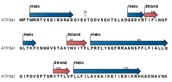
Example: Prediction of secondary structure from sequence
Dimensionality reduction and feature extraction
Unsupervised learning
input: high-dimensional data (e.g. MD simulations)
output: projection of data onto low-dimensional collective variable space
Example: Conformational clustering and identification of states sampled via MD

Generation of high-dimensional data
Supervised learning via advanced deep learning architectures
input: desired features of generated objects
output: ensembles of objects based on desired features and consistent with expected properties
Example: High-accuracy protein structure generation based on sequence

Models used in ML
In the most general sense, ML models map input data to output data.
\( \color{red}{Y}\color{black}{ = f(}\color{blue}{X}; \color{green}{W}; \color{purple}{P}; \color{grey}{N}\color{black}{)} \)
Model Input:
\( \begin{matrix} \color{blue}{\mbox{X}} & \mbox{input data} \\ \color{green}{\mbox{W}} & \mbox{weights to be optimized} \\ \color{purple}{\mbox{P}} & \mbox{model parameters} \\ \color{grey}{\mbox{N}} & \mbox{random noise (optional)} \\ \end{matrix} \)
The objective of ML is to find an optimal mapping based on training data and other prior knowledge.
Functional regression
Linear regression
\( y = ax + b \)
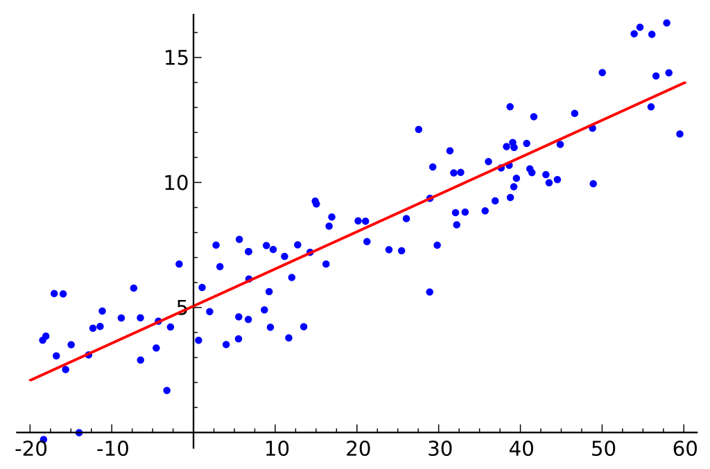
Uses: Prediction of continous value output
Logistic regression
Probability of observing certain outcome as a function of input \(x\):
\( \log(\frac{p}{1-p}) = \beta_0 + \beta_1*x \)

Uses: Classification
Support vector machines
The goal is to find a hyperplane that maximally separates data into two (or more) classes:
\( \textbf{w}^T \textbf{x} - b = 0 \)
with
\( \textbf{w}^T \textbf{x} - b \geq 1 \) for \( \color{blue}{\mbox{class 1}} \)
\( \textbf{w}^T \textbf{x} - b \leq 1 \) for \( \color{green}{\mbox{class 2}} \)
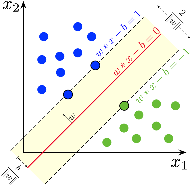
Uses: Classification
Decision Trees and Random Forests
Decision trees generete discrete outcomes from input data based on a series of ‘decisions’.
Random forest methods combine output from multiple decision trees based on random subsets of input data.

Uses: Classification

Neural Networks
Connect input to output via matrix operations and activation functions. Multiple network layers can be combined.

Uses: Regression, classification, analysis, encoding, generation

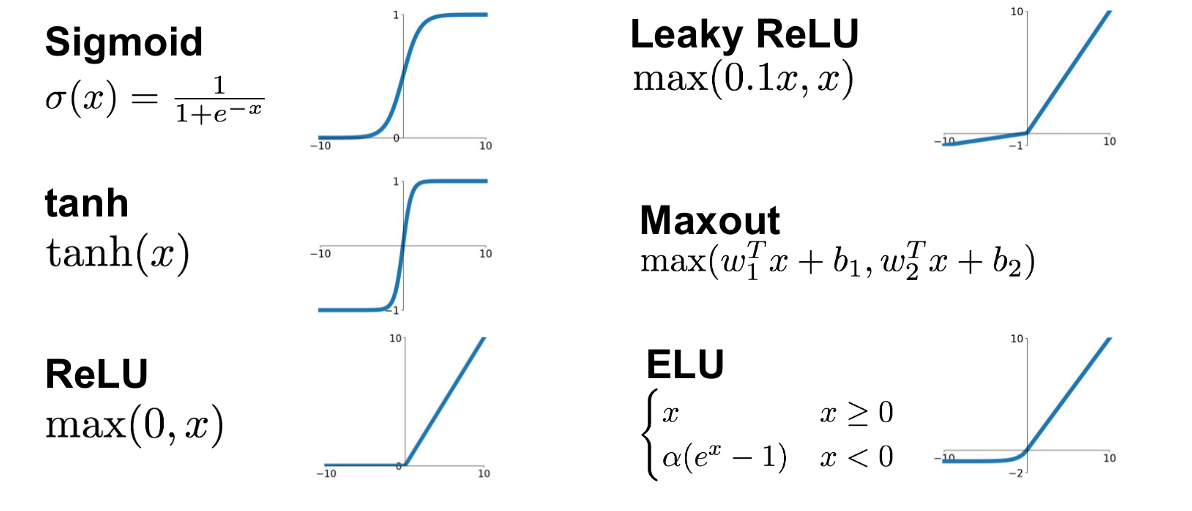
Activation functions
Activation functions are essential for modeling non-linear relationships and for gaining the full benefit of neural networks.
ML in practice
Define problem suitable for ML
What will be the input?
What will be the output?
What are the performance expectations?
Input data features
A good choice of input data features is essential for the success of machine learning.
general molecular properties (composition, mass, charge)
atomic coordinates (subject to rotational variance)
internal coordinates (distances, angles)
dynamic and ensemble information
sequences and multiple sequence alignments
classification based on previous knowledge
experimental data (e.g. density maps)
Target output data
The target output data should reflect the problem at hand and the availability of high-quality training data.
continuous values (e.g. energies, forces, molecular properties)
classification (e.g. secondary structure, topology, function)
latent space projection
embedding (encoding of data for further use)
distributions (e.g. distances, angles)
interactions (e.g. intra-/intermolecular contacts, ligands, ions)
structures (or parts of it)
dynamic ensembles (or aspects of dynamics)
quality assessment (e.g. model accuracy or experimental uncertainties)
Model design
The main consideration is the balance between model complexity, accuracy, and ease of training.
Neural networks are flexible and powerful but may be difficult to train
Deep networks may be more accurate and transferable but require more data
Deep networks are more difficulty to train than shallow models
Optimal model architecture should match input/output data shape (→ next week)
Computer hardware may limit model choices
Start from established models! (→ next week)
Model choices and hyper-parameters should be optimized as part of model training.
Model training
The goal of training a specific model is to find optimal weights.
This is the key step of machine learning that requires the most effort and computer resources.

How do we know which weights are optimal?
We define a loss function based on training data, e.g. MSE (mean-squared error) that should be minimized:
\(y_k(\textbf{x}_{k},\textbf{w},\textbf{p})\) is the model-predicted output given weights \(\textbf{w}\) and model parameters \(\textbf{p}\) for training data item \(k\).
\(\hat{y}_k\) is the expected output from the training data.
How do we find optimal weights?
We typically use a gradient descent minimizer (SGD: Stochastic Gradient Descent; Adam):

The minimizer updates weights iteratively according to: \(w_{new} = w_{old} - \lambda \frac{\partial J(w)}{\partial w} \)
\(\lambda\) is the learning rate and a key parameter that may be varied during optimization.
How do we obtain gradients?
Gradients are usually obtained via back-propagation, i.e. application of the chain rule.

When do we stop with training?
When the loss function stops decreasing.
It is better to monitor model performance on a validation set and stop when loss function on validation set starts to increase (indicates overfitting).

How do we optimize training performance?
Use GPUs or TPUs with lots of memory.
Batch processing to manage large training data sets.
Adaptive learning rate (start slow, faster steps once optimization converges)
Use pre-trained models and apply transfer learning
Explore different model architectures and different activation functions
Regularize input data (training is easiest with values in 0-1 range)
Data
Data is critical for machine learning. The data should provide reliable mappings between input features and target output data from which a model can be learned.
To develop rigorous models, data should be divided into three sets:
training data (70-90%): these data are used directly for training the model
validation data (10-30%): these data are used for testing model performance during training to determine when to stop and to optimize hyper-parameters
test data: these (separate) data are used for evaluating the accuracy of the final models and may consist of benchmarks that allow comparison with other methods or reference data from physical theory or experiments
Splitting the initial data into training and validation sets should be repeated randomly.
Data biases and incorporation of additional knowledge
ML models perform best on domains covered extensively input data and transfer poorly to other scenarios where no or little training data was available.
To prevent bias, training data should uniformly cover the broadest possible range of scenarios.
Data augmentation may provide additional data for areas not well-covered initially, e.g. for trivial cases.
Training data may be supplemented by constraints based on other knowledge that can be applied during training, e.g. physical constraints that disallow atom overlap or negative output values for properties that can only assume positive values.
Using ML models
Once we have a trained model, the model is easy to apply. All we need is the model architecture and the trained weights.
Forward evaluation is usually very fast, but can take time (and require GPU resources) for very large models. More significant time may be needed for generating the required input features (e.g. multiple sequence alignments as input to AlphaFold2).
The usefulness of a given ML model greatly depends on the training data. If the training data is limited, the model, transferability (and broader use) is probably also limited.
Validation of a given ML model is critical for understanding its expected accuracy.
Interpreting ML models
ML models are designed to make highly accurate predictions. That may be sufficient.
What if we want to understand things?
Direct inspection of optimized weights is usually not productive. Most models are too complex.
More insights can be gained from ablation studies that remove input features one-by-one to analyze how the model performance after training changes.
It may also be possible to gain insights into what information is contained in the training data by challenging the trained model with unexpected input data.